How to Make Graph Paper in Excel
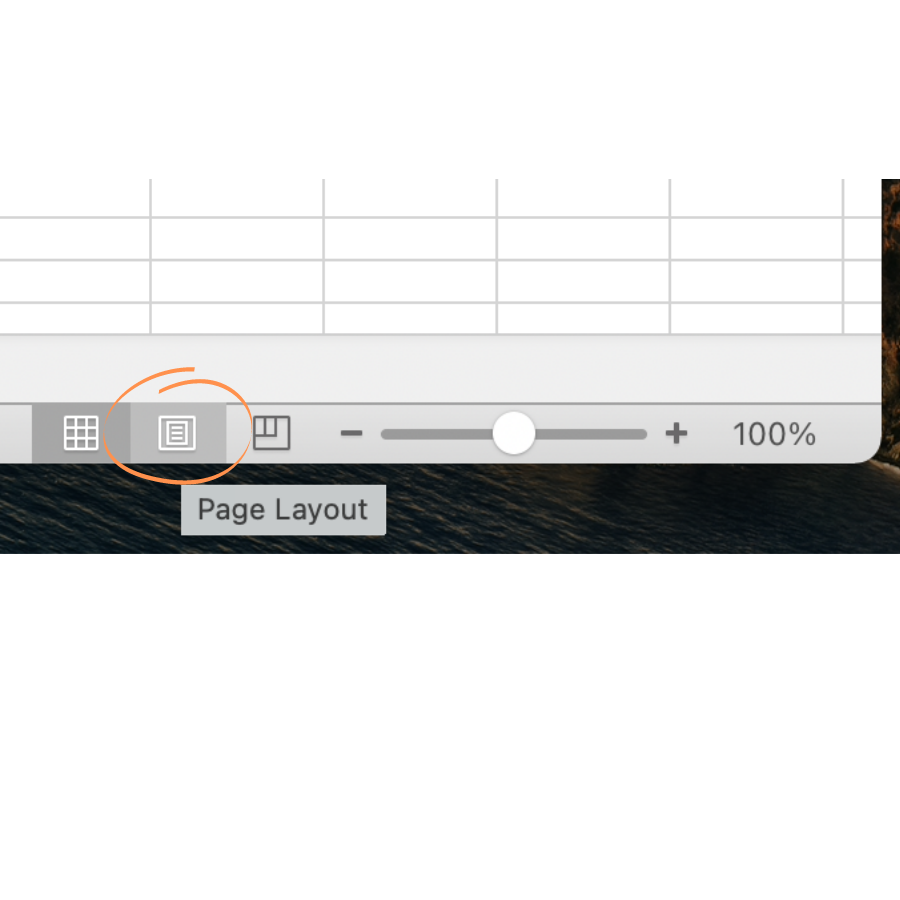
Step 1. Change to “Page Layout” View
Open a new empty Excel sheet. In the bottom right hand corner of the sheet, select the ‘Page Layout’ view. Your Excel sheet should now look like separate pages of paper rather than one large grid.
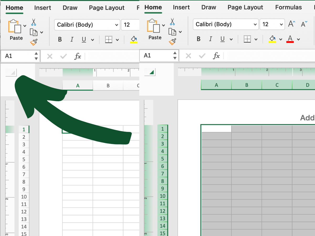
Step 2. Select all cells
In the upper left corner of the sheet select the half triangle button. When this button is pressed all the cells should be highlighted.

Step 3. Format the Column Width
While all the cells are highlighted, click on the vertical bar in between columns ‘A’ and ‘B’. Drag the line left and right to make the cell narrower or wider. A measurement should appear telling you what the current measurement of the block is in inches.
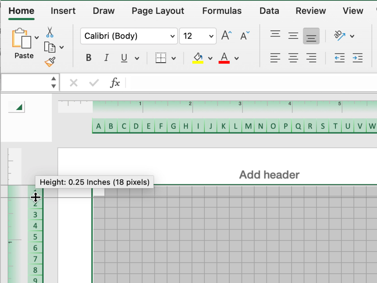
Step 4. Adjust the Row Height
While all the cells are highlighted (see Step 2) click on the horizontal bar between the row ‘1’ and ‘2’ labels. Drag this line up and down to make the cells narrower or wider. To create a perfect square, drag the box until the measurement matches what you selected for the column width.

Step 5. Return to ‘Normal’ Page View (Optional)
To return to the ‘Normal’ page view, select the grid button in the bottom right hand toolbar of the Excel window.